目录
- tensorflow是非常强的工具,生态庞大
- tensorflow提供了Keras的分支
- Define tensor constants.
- Linear Regression
- 分类模型
- 本例使用MNIST手写数字
- Model prediction: 7
- Model prediction: 2
- Model prediction: 1
- Model prediction: 0
- Model prediction: 4
TF 目前发布2.5 版本,之前阅读1.X官方文档,最近查看2.X的文档。
tensorflow是非常强的工具,生态庞大
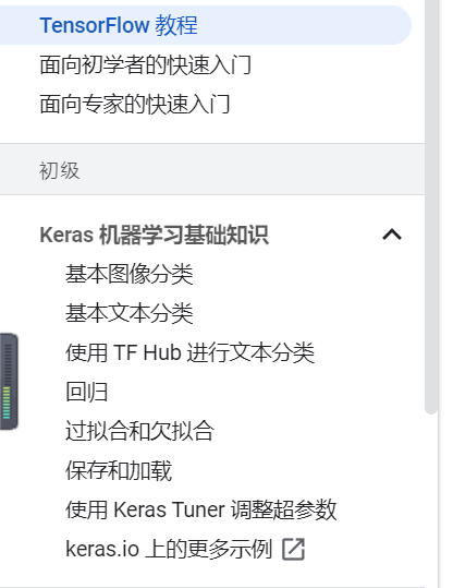
tensorflow提供了Keras的分支
这里不再提供Keras相关顺序模型教程。
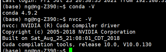
关于环境:ubuntu的 GPU,需要cuda和nvcc
不会安装:查看
完整的Ubuntu18.04深度学习GPU环境配置,英伟达显卡驱动安装、cuda9.0安装、cudnn的安装、anaconda安装
不安装,直接翻墙用colab
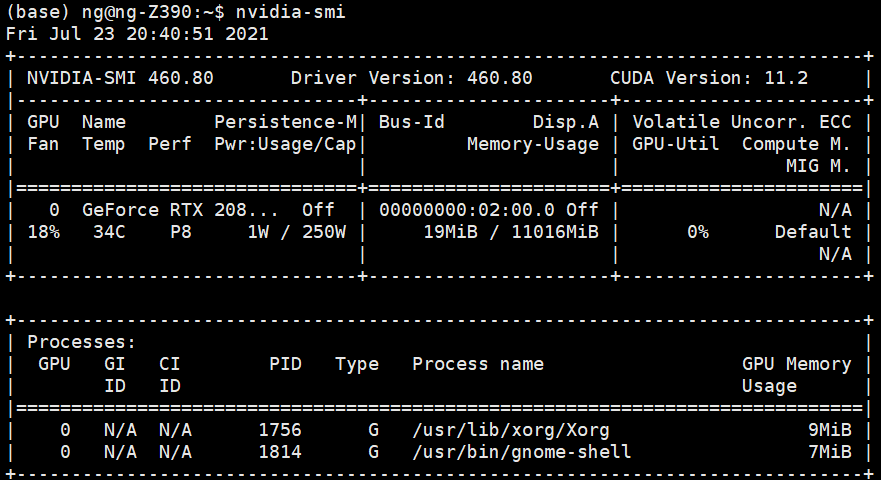
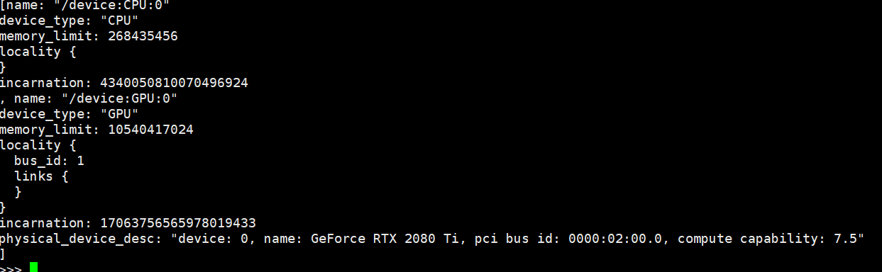
测试GPU
>>> from tensorflow.python.client import device_lib
>>> device_lib.list_local_devices()
这是意思是挂了一个显卡
具体查看官方文档:https://www.tensorflow.org/install
服务器跑Jupyter
Define tensor constants.
import tensorflow as tf
# Create a Tensor.
hello = tf.constant("hello world")
hello
# Define tensor constants.
a = tf.constant(1)
b = tf.constant(6)
c = tf.constant(9)
# tensor变量的操作
# (+, *, ...)
add = tf.add(a, b)
sub = tf.subtract(a, b)
mul = tf.multiply(a, b)
div = tf.divide(a, b)
# 通过numpy返回数值  和torch一样
print("add =", add.numpy())
print("sub =", sub.numpy())
print("mul =", mul.numpy())
print("div =", div.numpy())
add = 7
sub = -5
mul = 6
div = 0.16666666666666666
mean = tf.reduce_mean([a, b, c])
sum_ = tf.reduce_sum([a, b, c])
# Access tensors value.
print("mean =", mean.numpy())
print("sum =", sum_ .numpy())
mean = 5
sum = 16
# Matrix multiplications.
matrix1 = tf.constant([[1., 2.], [3., 4.]])
matrix2 = tf.constant([[5., 6.], [7., 8.]])
product = tf.matmul(matrix1, matrix2)
product
tf.Tensor: shape=(2, 2), dtype=float32, numpy=
array([[19., 22.],
       [43., 50.]], dtype=float32)>
# Tensor to Numpy.
np_product = product.numpy()
print(type(np_product), np_product)
(numpy.ndarray,
 array([[19., 22.],
        [43., 50.]], dtype=float32))
Linear Regression
下面使用tensorflow快速构建线性回归模型,这里不使用kears的顺序模型,而是采用torch的模型定义的写法。
import numpy as np
import tensorflow as tf
# Parameters:
learning_rate = 0.01
training_steps = 1000
display_step = 50
# Training Data.
X = np.array([3.3,4.4,5.5,6.71,6.93,4.168,9.779,6.182,7.59,2.167,7.042,10.791,5.313,7.997,5.654,9.27,3.1])
Y = np.array([1.7,2.76,2.09,3.19,1.694,1.573,3.366,2.596,2.53,1.221,2.827,3.465,1.65,2.904,2.42,2.94,1.3])
random = np.random
# 权重和偏差,随机初始化。
W = tf.Variable(random.randn(), name="weight")
b = tf.Variable(random.randn(), name="bias")
# Linear regression (Wx + b).
def linear_regression(x):
return W * x + b
# Mean square error.
def mean_square(y_pred, y_true):
return tf.reduce_mean(tf.square(y_pred - y_true))
# 随机梯度下降优化器。
optimizer = tf.optimizers.SGD(learning_rate)
# 优化过程。
def run_optimization():
# 将计算包在GradientTape中,以便自动区分。
with tf.GradientTape() as g:
pred = linear_regression(X)
loss = mean_square(pred, Y)
# 计算梯度。
gradients = g.gradient(loss, [W, b])
# 按照梯度更新W和b。
optimizer.apply_gradients(zip(gradients, [W, b]))
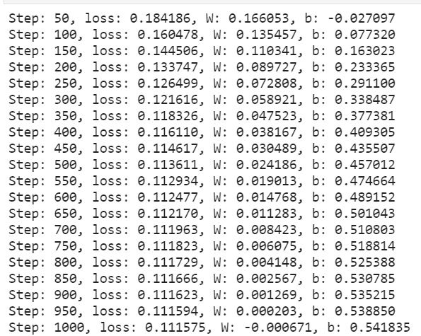
#按给定的步数进行训练。
for step in range(1, training_steps + 1):
# 运行优化以更新W和b值。
run_optimization()
if step % display_step == 0:
pred = linear_regression(X)
loss = mean_square(pred, Y)
print("Step: %i, loss: %f, W: %f, b: %f" % (step, loss, W.numpy(), b.numpy()))
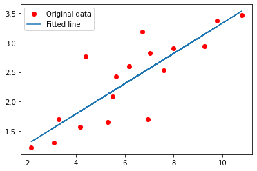
import matplotlib.pyplot as plt
plt.plot(X, Y, 'ro', label='Original data')
plt.plot(X, np.array(W * X + b), label='Fitted line')
plt.legend()
plt.show()
分类模型
本例使用MNIST手写数字
数据集包含60000个训练示例和10000个测试示例。
这些数字已经过大小标准化,并在一个固定大小的图像(28x28像素)中居中,值从0到255。
在本例中,每个图像将转换为float32,标准化为[0,1],并展平为784个特征(28×28)的一维数组。
import numpy as np
import tensorflow as tf
# MNIST data
num_classes = 10 # 0->9 digits
num_features = 784 # 28 * 28
# Parameters
lr = 0.01
batch_size = 256
display_step = 100
training_steps = 1000
# Prepare MNIST data
from tensorflow.keras.datasets import mnist
(x_train, y_train), (x_test, y_test) = mnist.load_data()
# Convert to Float32
x_train, x_test = np.array(x_train, np.float32), np.array(x_test, np.float32)
# Flatten images into 1-D vector of 784 dimensions (28 * 28)
x_train, x_test = x_train.reshape([-1, num_features]), x_test.reshape([-1, num_features])
# [0, 255] to [0, 1]
x_train, x_test = x_train / 255, x_test / 255
# 打乱顺序: tf.data API to shuffle and batch data
train_dataset = tf.data.Dataset.from_tensor_slices((x_train, y_train))
train_dataset = train_dataset.repeat().shuffle(5000).batch(batch_size=batch_size).prefetch(1)
# Weight of shape [784, 10] ~= [number_features, number_classes]
W = tf.Variable(tf.ones([num_features, num_classes]), name='weight')
# Bias of shape [10] ~= [number_classes]
b = tf.Variable(tf.zeros([num_classes]), name='bias')
# Logistic regression: W*x + b
def logistic_regression(x):
# 应用softmax函数将logit标准化为概率分布
out = tf.nn.softmax(tf.matmul(x, W) + b)
return out
# 交叉熵损失函数
def cross_entropy(y_pred, y_true):
# 将标签编码为一个one_hot向量
y_true = tf.one_hot(y_true, depth=num_classes)
# 剪裁预测值避免错误
y_pred = tf.clip_by_value(y_pred, 1e-9, 1)
# 计算交叉熵
cross_entropy = tf.reduce_mean(-tf.reduce_sum(y_true * tf.math.log(y_pred), 1))
return cross_entropy
# Accuracy
def accuracy(y_pred, y_true):
correct = tf.equal(tf.argmax(y_pred, 1), tf.cast(y_true, tf.int64))
return tf.reduce_mean(tf.cast(correct, tf.float32))
# 随机梯度下降优化器
optimizer = tf.optimizers.SGD(lr)
# Optimization
def run_optimization(x, y):
with tf.GradientTape() as g:
pred = logistic_regression(x)
loss = cross_entropy(y_pred=pred, y_true=y)
gradients = g.gradient(loss, [W, b])
optimizer.apply_gradients(zip(gradients, [W, b]))
# Training
for step, (batch_x, batch_y) in enumerate(train_dataset.take(training_steps), 1):
# Run the optimization to update W and b
run_optimization(x=batch_x, y=batch_y)
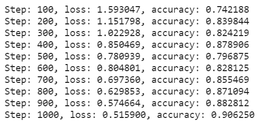
if step % display_step == 0:
pred = logistic_regression(batch_x)
loss = cross_entropy(y_pred=pred, y_true=batch_y)
acc = accuracy(y_pred=pred, y_true=batch_y)
print("Step: %i, loss: %f, accuracy: %f" % (step, loss, acc))
pred = logistic_regression(x_test)
print(f"Test Accuracy: {accuracy(pred, y_test)}")
Test Accuracy: 0.892300009727478
import matplotlib.pyplot as plt
n_images = 5
test_images = x_test[:n_images]
predictions = logistic_regression(test_images)
# 预测前5张
for i in range(n_images):
    plt.imshow(np.reshape(test_images[i], [28, 28]), cmap='gray')
    plt.show()
    print("Model prediction: %i" % np.argmax(predictions.numpy()[i]))
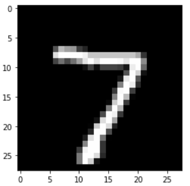
Model prediction: 7
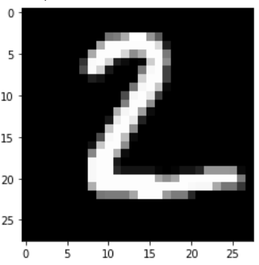
Model prediction: 2
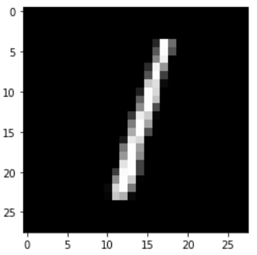
Model prediction: 1
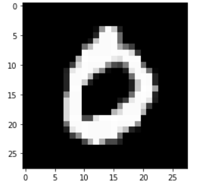
Model prediction: 0
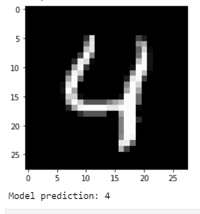
Model prediction: 4
以上就是tensorflow基本操作小白快速构建线性回归和分类模型的详细内容,更多关于tensorflow快速构建线性回归和分类模型的资料请关注脚本之家其它相关文章!
您可能感兴趣的文章:- tensorflow入门之训练简单的神经网络方法
- TensorFlow使用Graph的基本操作的实现
- 详解tensorflow实现迁移学习实例
- Python深度学习TensorFlow神经网络基础概括


 咨 询 客 服