详解TensorFlow2实现前向传播-巨人网络通讯

详解TensorFlow2实现前向传播

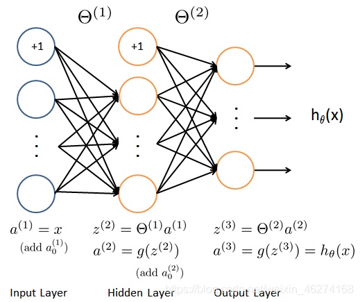
概述

前向传播 (Forward propagation) 是将上一层输出作为下一层的输入, 并计算下一层的输出, 一直到运算到输出层为止.

会用到的函数

张量最小值

```reduce_min``函数可以帮助我们计算一个张量各个维度上元素的最小值.

格式:

tf.math.reduce_min(
    input_tensor, axis=None, keepdims=False, name=None
)

参数:

input_tensor: 传入的张量
axis: 维度, 默认计算所有维度
keepdims: 如果为真保留维度, 默认为 False
name: 数据名称

张量最大值

```reduce_max``函数可以帮助我们计算一个张量各个维度上元素的最大值.

格式:

tf.math.reduce_max(
    input_tensor, axis=None, keepdims=False, name=None
)

参数:

input_tensor: 传入的张量
axis: 维度, 默认计算所有维度
keepdims: 如果为真保留维度, 默认为 False
name: 数据名称

数据集分批

from_tensor_slices可以帮助我们切分传入 Tensor 的第一个维度. 得到的每个切片都是一个样本数据.

格式:

@staticmethod
from_tensor_slices(
    tensors
)

迭代

我们可以调用iter函数来生成迭代器.

格式:

iter(object[, sentinel])

参数:
-object: 支持迭代的集合对象

sentinel: 如果传递了第二个参数, 则参数 object 必须是一个可调用的对象 (如, 函数). 此时, iter 创建了一个迭代器对象, 每次调用这个迭代器对象的__next__()方法时, 都会调用 object

例子:

list = [1, 2, 3]
i = iter(list)
print(next(i))
print(next(i))
print(next(i))

输出结果:

1
2
3

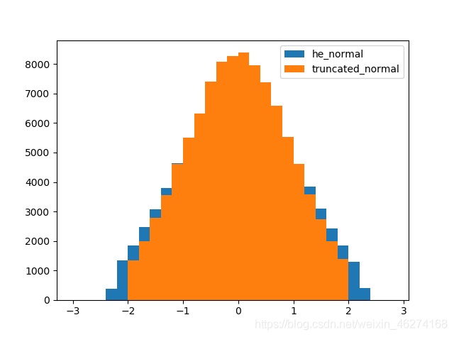
截断正态分布

truncated_normal可以帮助我们生成一个截断的正态分布. 生成的正态分布值会在两倍的标准差的范围之内.

格式:

tf.random.truncated_normal(
    shape, mean=0.0, stddev=1.0, dtype=tf.dtypes.float32, seed=None, name=None
)

参数:

shape: 张量的形状
mean: 正态分布的均值, 默认 0.0
stddev: 正态分布的标准差, 默认为 1.0
dtype: 数据类型, 默认为 float32
seed: 随机数种子
name: 数据名称

relu 激活函数

激活函数有 sigmoid, maxout, relu 等等函数. 通过激活函数我们可以使得各个层之间达成非线性关系.

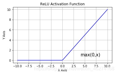
激活函数可以帮助我们提高模型健壮性, 提高非线性表达能力, 缓解梯度消失问题.

one_hot

tf.one_hot函数是讲 input 准换为 one_hot 类型数据输出. 相当于将多个数值联合放在一起作为多个相同类型的向量.

格式:

tf.one_hot(
    indices, depth, on_value=None, off_value=None, axis=None, dtype=None, name=None
)

参数:

indices: 索引的张量
depth: 指定独热编码维度的标量
on_value: 索引 indices[j] = i 位置处填充的标量，默认为 1
off_value: 索引 indices[j] != i 所有位置处填充的标量, 默认为 0
axis: 填充的轴, 默认为 -1 (最里面的新轴)
dtype: 输出张量的数据格式
name：数据名称

assign_sub

assign_sub可以帮助我们实现张量自减.

格式:

tf.compat.v1.assign_sub(
    ref, value, use_locking=None, name=None
)

参数:

ref: 多重张量
value: 张量
use_locking: 锁
name: 数据名称

准备工作

import tensorflow as tf

# 定义超参数
batch_size = 256  # 一次训练的样本数目
learning_rate = 0.001  # 学习率
iteration_num = 20  # 迭代次数

# 读取mnist数据集
(x, y), _ = tf.keras.datasets.mnist.load_data()  # 读取训练集的特征值和目标值
print(x[:5])  # 调试输出前5个图
print(y[:5])  # 调试输出前5个目标值数字
print(x.shape)  # (60000, 28, 28) 单通道
print(y.shape)  # (60000,)

# 转换成常量tensor
x = tf.convert_to_tensor(x, dtype=tf.float32) / 255  # 转换为0~1的形式
y = tf.convert_to_tensor(y, dtype=tf.int32)  # 转换为整数形式

# 调试输出范围
print(tf.reduce_min(x), tf.reduce_max(x))  # 0~1
print(tf.reduce_min(y), tf.reduce_max(y))  # 0~9

# 分割数据集
train_db = tf.data.Dataset.from_tensor_slices((x, y)).batch(batch_size)  # 256为一个batch
train_iter = iter(train_db)  # 生成迭代对象

# 定义权重和bias [256, 784] => [256, 256] => [256, 128] => [128, 10]
w1 = tf.Variable(tf.random.truncated_normal([784, 256], stddev=0.1))  # 标准差为0.1的截断正态分布
b1 = tf.Variable(tf.zeros([256]))  # 初始化为0

w2 = tf.Variable(tf.random.truncated_normal([256, 128], stddev=0.1))  # 标准差为0.1的截断正态分布
b2 = tf.Variable(tf.zeros([128]))  # 初始化为0

w3 = tf.Variable(tf.random.truncated_normal([128, 10], stddev=0.1))  # 标准差为0.1的截断正态分布
b3 = tf.Variable(tf.zeros([10]))  # 初始化为0

输出结果:

[[[0 0 0 ... 0 0 0]
[0 0 0 ... 0 0 0]
[0 0 0 ... 0 0 0]
...
[0 0 0 ... 0 0 0]
[0 0 0 ... 0 0 0]
[0 0 0 ... 0 0 0]]

[[0 0 0 ... 0 0 0]
[0 0 0 ... 0 0 0]
[0 0 0 ... 0 0 0]
...
[0 0 0 ... 0 0 0]
[0 0 0 ... 0 0 0]
[0 0 0 ... 0 0 0]]

[[0 0 0 ... 0 0 0]
[0 0 0 ... 0 0 0]
[0 0 0 ... 0 0 0]
...
[0 0 0 ... 0 0 0]
[0 0 0 ... 0 0 0]
[0 0 0 ... 0 0 0]]

[[0 0 0 ... 0 0 0]
[0 0 0 ... 0 0 0]
[0 0 0 ... 0 0 0]
...
[0 0 0 ... 0 0 0]
[0 0 0 ... 0 0 0]
[0 0 0 ... 0 0 0]]

[[0 0 0 ... 0 0 0]
[0 0 0 ... 0 0 0]
[0 0 0 ... 0 0 0]
...
[0 0 0 ... 0 0 0]
[0 0 0 ... 0 0 0]
[0 0 0 ... 0 0 0]]]
[5 0 4 1 9]
(60000, 28, 28)
(60000,)
tf.Tensor(0.0, shape=(), dtype=float32) tf.Tensor(1.0, shape=(), dtype=float32)
tf.Tensor(0, shape=(), dtype=int32) tf.Tensor(9, shape=(), dtype=int32)

train 函数

def train(epoch):  # 训练
    for step, (x, y) in enumerate(train_db):  # 每一批样本遍历
        # 把x平铺 [256, 28, 28] => [256, 784]
        x = tf.reshape(x, [-1, 784])

        with tf.GradientTape() as tape:  # 自动求解
            # 第一个隐层 [256, 784] => [256, 256]
            # [256, 784]@[784, 256] + [256] => [256, 256] + [256] => [256, 256] + [256, 256] (广播机制)
            h1 = x @ w1 + tf.broadcast_to(b1, [x.shape[0], 256])
            h1 = tf.nn.relu(h1)  # relu激活

            # 第二个隐层 [256, 256] => [256, 128]
            h2 = h1 @ w2 + b2
            h2 = tf.nn.relu(h2)  # relu激活

            # 输出层 [256, 128] => [128, 10]
            out = h2 @ w3 + b3

            # 计算损失MSE(Mean Square Error)
            y_onehot = tf.one_hot(y, depth=10)  # 转换成one_hot编码
            loss = tf.square(y_onehot - out)  # 计算总误差
            loss = tf.reduce_mean(loss)  # 计算平均误差MSE


        # 计算梯度
        grads = tape.gradient(loss, [w1, b1, w2, b2, w3, b3])

        # 更新权重
        w1.assign_sub(learning_rate * grads[0])  # 自减梯度*学习率
        b1.assign_sub(learning_rate * grads[1])  # 自减梯度*学习率
        w2.assign_sub(learning_rate * grads[2])  # 自减梯度*学习率
        b2.assign_sub(learning_rate * grads[3])  # 自减梯度*学习率
        w3.assign_sub(learning_rate * grads[4])  # 自减梯度*学习率
        b3.assign_sub(learning_rate * grads[5])  # 自减梯度*学习率

        if step % 100 == 0:  # 每运行100个批次, 输出一次
            print("epoch:", epoch, "step:", step, "loss:", float(loss))

run 函数

def run():
    for i in range(iteration_num):  # 迭代20次
        train(i)

完整代码

import tensorflow as tf

# 定义超参数
batch_size = 256  # 一次训练的样本数目
learning_rate = 0.001  # 学习率
iteration_num = 20  # 迭代次数

# 读取mnist数据集
(x, y), _ = tf.keras.datasets.mnist.load_data()  # 读取训练集的特征值和目标值
print(x[:5])  # 调试输出前5个图
print(y[:5])  # 调试输出前5个目标值数字
print(x.shape)  # (60000, 28, 28) 单通道
print(y.shape)  # (60000,)

# 转换成常量tensor
x = tf.convert_to_tensor(x, dtype=tf.float32) / 255  # 转换为0~1的形式
y = tf.convert_to_tensor(y, dtype=tf.int32)  # 转换为整数形式

# 调试输出范围
print(tf.reduce_min(x), tf.reduce_max(x))  # 0~1
print(tf.reduce_min(y), tf.reduce_max(y))  # 0~9

# 分割数据集
train_db = tf.data.Dataset.from_tensor_slices((x, y)).batch(batch_size)  # 256为一个batch
train_iter = iter(train_db)  # 生成迭代对象

# 定义权重和bias [256, 784] => [256, 256] => [256, 128] => [128, 10]
w1 = tf.Variable(tf.random.truncated_normal([784, 256], stddev=0.1))  # 标准差为0.1的截断正态分布
b1 = tf.Variable(tf.zeros([256]))  # 初始化为0

w2 = tf.Variable(tf.random.truncated_normal([256, 128], stddev=0.1))  # 标准差为0.1的截断正态分布
b2 = tf.Variable(tf.zeros([128]))  # 初始化为0

w3 = tf.Variable(tf.random.truncated_normal([128, 10], stddev=0.1))  # 标准差为0.1的截断正态分布
b3 = tf.Variable(tf.zeros([10]))  # 初始化为0


def train(epoch):  # 训练
    for step, (x, y) in enumerate(train_db):  # 每一批样本遍历
        # 把x平铺 [256, 28, 28] => [256, 784]
        x = tf.reshape(x, [-1, 784])

        with tf.GradientTape() as tape:  # 自动求解
            # 第一个隐层 [256, 784] => [256, 256]
            # [256, 784]@[784, 256] + [256] => [256, 256] + [256] => [256, 256] + [256, 256] (广播机制)
            h1 = x @ w1 + tf.broadcast_to(b1, [x.shape[0], 256])
            h1 = tf.nn.relu(h1)  # relu激活

            # 第二个隐层 [256, 256] => [256, 128]
            h2 = h1 @ w2 + b2
            h2 = tf.nn.relu(h2)  # relu激活

            # 输出层 [256, 128] => [128, 10]
            out = h2 @ w3 + b3

            # 计算损失MSE(Mean Square Error)
            y_onehot = tf.one_hot(y, depth=10)  # 转换成one_hot编码
            loss = tf.square(y_onehot - out)  # 计算总误差
            loss = tf.reduce_mean(loss)  # 计算平均误差MSE


        # 计算梯度
        grads = tape.gradient(loss, [w1, b1, w2, b2, w3, b3])

        # 更新权重
        w1.assign_sub(learning_rate * grads[0])  # 自减梯度*学习率
        b1.assign_sub(learning_rate * grads[1])  # 自减梯度*学习率
        w2.assign_sub(learning_rate * grads[2])  # 自减梯度*学习率
        b2.assign_sub(learning_rate * grads[3])  # 自减梯度*学习率
        w3.assign_sub(learning_rate * grads[4])  # 自减梯度*学习率
        b3.assign_sub(learning_rate * grads[5])  # 自减梯度*学习率

        if step % 100 == 0:  # 每运行100个批次, 输出一次
            print("epoch:", epoch, "step:", step, "loss:", float(loss))


def run():
    for i in range(iteration_num):  # 迭代20次
        train(i)


if __name__ == "__main__":
    run()

输出结果:

epoch: 0 step: 0 loss: 0.5439826250076294
epoch: 0 step: 100 loss: 0.2263326346874237
epoch: 0 step: 200 loss: 0.19458135962486267
epoch: 1 step: 0 loss: 0.1788959801197052
epoch: 1 step: 100 loss: 0.15782299637794495
epoch: 1 step: 200 loss: 0.1580992043018341
epoch: 2 step: 0 loss: 0.15085121989250183
epoch: 2 step: 100 loss: 0.1432340145111084
epoch: 2 step: 200 loss: 0.14373672008514404
epoch: 3 step: 0 loss: 0.13810500502586365
epoch: 3 step: 100 loss: 0.13337770104408264
epoch: 3 step: 200 loss: 0.1334681361913681
epoch: 4 step: 0 loss: 0.12887853384017944
epoch: 4 step: 100 loss: 0.12551936507225037
epoch: 4 step: 200 loss: 0.125375896692276
epoch: 5 step: 0 loss: 0.12160968780517578
epoch: 5 step: 100 loss: 0.1190723180770874
epoch: 5 step: 200 loss: 0.11880680173635483
epoch: 6 step: 0 loss: 0.11563797295093536
epoch: 6 step: 100 loss: 0.11367204040288925
epoch: 6 step: 200 loss: 0.11331651359796524
epoch: 7 step: 0 loss: 0.11063456535339355
epoch: 7 step: 100 loss: 0.10906648635864258
epoch: 7 step: 200 loss: 0.10866570472717285
epoch: 8 step: 0 loss: 0.10636782646179199
epoch: 8 step: 100 loss: 0.10510052740573883
epoch: 8 step: 200 loss: 0.10468046367168427
epoch: 9 step: 0 loss: 0.10268573462963104
epoch: 9 step: 100 loss: 0.10163718461990356
epoch: 9 step: 200 loss: 0.10121693462133408
epoch: 10 step: 0 loss: 0.09949333965778351
epoch: 10 step: 100 loss: 0.09859145432710648
epoch: 10 step: 200 loss: 0.09819269925355911
epoch: 11 step: 0 loss: 0.0966767817735672
epoch: 11 step: 100 loss: 0.09586615860462189
epoch: 11 step: 200 loss: 0.09550992399454117
epoch: 12 step: 0 loss: 0.09417577087879181
epoch: 12 step: 100 loss: 0.09341947734355927
epoch: 12 step: 200 loss: 0.09310202300548553
epoch: 13 step: 0 loss: 0.09193204343318939
epoch: 13 step: 100 loss: 0.09122277796268463
epoch: 13 step: 200 loss: 0.09092779457569122
epoch: 14 step: 0 loss: 0.0899026170372963
epoch: 14 step: 100 loss: 0.08923697471618652
epoch: 14 step: 200 loss: 0.08895798027515411
epoch: 15 step: 0 loss: 0.08804921805858612
epoch: 15 step: 100 loss: 0.08742769062519073
epoch: 15 step: 200 loss: 0.0871589332818985
epoch: 16 step: 0 loss: 0.08635203540325165
epoch: 16 step: 100 loss: 0.0857706069946289
epoch: 16 step: 200 loss: 0.0855005756020546
epoch: 17 step: 0 loss: 0.08479145169258118
epoch: 17 step: 100 loss: 0.08423925191164017
epoch: 17 step: 200 loss: 0.08396687358617783
epoch: 18 step: 0 loss: 0.08334997296333313
epoch: 18 step: 100 loss: 0.08281457424163818
epoch: 18 step: 200 loss: 0.08254452794790268
epoch: 19 step: 0 loss: 0.08201286941766739
epoch: 19 step: 100 loss: 0.08149122446775436
epoch: 19 step: 200 loss: 0.08122102916240692