一、Python图像处理PIL库
1.1 转换图像格式
# PIL(Python Imaging Library)
from PIL import Image
plt.rcParams['font.sans-serif'] = ['SimHei']
# 读取的是图像,cv.imread读取的是array,Image.open()显示的图像是RGB
pil_im=Image.open('pic/kobe_mamba.jpg')

subplot(121),plt.title('原图'),axis('off')
imshow(pil_im)

pil_im_gray=pil_im.convert('L')
subplot(122),plt.title('灰度图'),xticks(x,()),yticks(y,())
imshow(pil_im_gray)

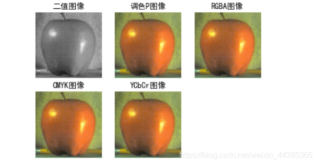
# 转换图像格式 PIL中有九种不同模式。分别为1,L,P,RGB,RGBA,CMYK,YCbCr,I,F。
import matplotlib.pyplot as plt
import numpy as np
from PIL import Image
plt.rcParams['font.sans-serif'] = ['SimHei']

pil_im=Image.open('pic/apple.jpg')

# 模式1 二值图像

pil_im_binary=pil_im.convert('1')
subplot(231),plt.title('二值图像'),axis('off'),imshow(pil_im_binary)

pil_im_binary.getpixel((10,10))

# 模式2 L = R * 299/1000 + G * 587/1000+ B * 114/1000 灰度模式 0表示黑,255表示白

# 模式3 P模式为8位彩色图像,通过RGB调色

pil_im_p=pil_im.convert('P')

subplot(232),plt.title('调色P图像'),axis('off'),imshow(pil_im_p)

# 模式4 模式“RGBA”为32位彩色图像,它的每个像素用32个bit表示,其中24bit表示红色、绿色和蓝色三个通道,另外8bit(255)表示alpha通道,255表示不透明。

pil_im_RGBA=pil_im.convert('RGBA')

subplot(233),plt.title('RGBA图像'),axis('off'),imshow(pil_im_RGBA)

# 模式5 CMYK 三原色+黑色,每个像素由32位表示
# C = 255 - R, M = 255 - G, Y = 255 - B, K = 0

pil_im_CMYK=pil_im.convert('CMYK')

subplot(234),plt.title('CMYK图像'),axis('off'),imshow(pil_im_CMYK)

#模式6 YCbcr 24位bit表示 Y= 0.257*R+0.504*G+0.098*B+16 Cb = -0.148*R-0.291*G+0.439*B+128 Cr = 0.439*R-0.368*G-0.071*B+128

pil_im_YCbCr=pil_im.convert('YCbCr')

subplot(235),plt.title('YCbCr图像'),axis('off'),imshow(pil_im_YCbCr)

# 模式7 I模式略 与L模式显示相同 ,只不过是32bit

# 模式8 F模式略 像素保留小数,其余与L模式相同
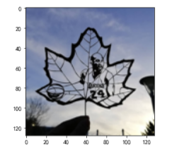
1.2 缩略图
# PIL(Python Imaging Library)
from PIL import Image
from pylab import *
plt.rcParams['font.sans-serif'] = ['SimHei']

pil_im=Image.open('pic/kobe_mamba.jpg')


# 创建缩略图 且可以指定大小

pil_im.thumbnail((120,120))

plt.title('缩略图'),xticks(x,()),yticks([])
imshow(pil_im)

1.3 复制、粘贴和旋转、调整尺寸
# 元组坐标分别为(左、上、右、下),从而标出了一块区域,相当于[100:400,100:400]

box=(100,100,400,400)

region=pil_im.crop(box)
# 旋转180度
region=region.transpose(Image.ROTATE_180)

figure(figsize=(5,5))

plt.title('复制区域'),axis('off')


imshow(region)
#粘贴


pil_im=Image.open('pic/kobe_mamba.jpg')

pil_im.paste(region,box)

figure(figsize=(5,5))

plt.title('粘贴后的图像'),axis('off')

imshow(pil_im)

# 调整尺寸和旋转 resize 和 rotate 函数

out=pil_im.resize((128,128))

out=pil_im.rotate(45)
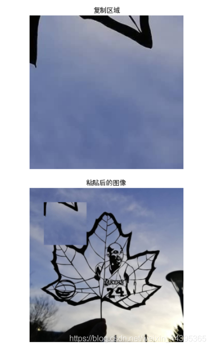
第二张图是box旋转了180度再粘贴的结果
二、Matoplotlib库基础学习
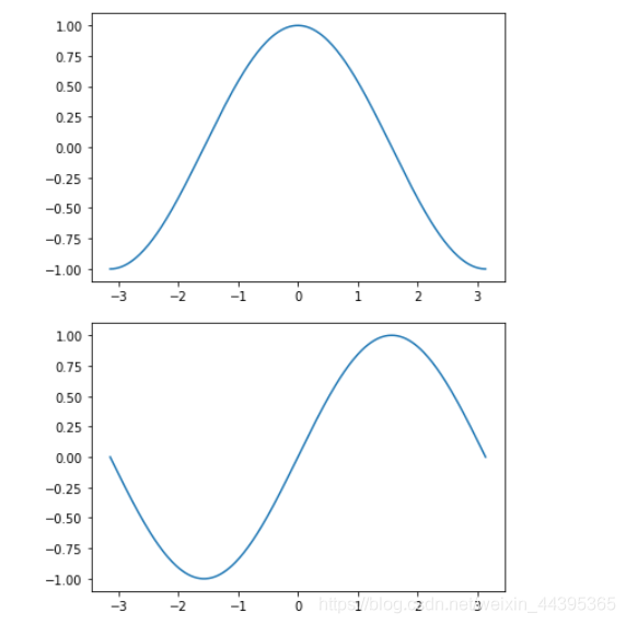
# 基本绘图
import numpy as np
import matplotlib.pyplot as plt
from numpy import pi
from pylab import *

x=np.linspace(-pi,pi,256)
y,z=np.cos(x),np.sin(x)
figure()
plt.plot(x,y)
figure()
plt.plot(x,z)
plt.show()
两张绘图
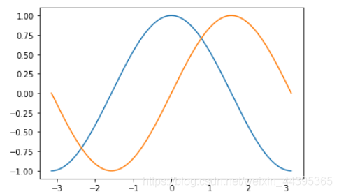
x=np.linspace(-pi,pi,256)
y,z=np.cos(x),np.sin(x)
plt.plot(x,y)
plt.plot(x,z)
绘图叠加
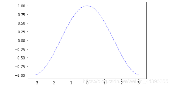
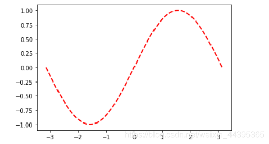
# 曲线颜色、标记、粗细
plot(x, y, color="blue", linewidth=1.0, linestyle=":")
plot(x,z,'--r',linewidth=2.0)
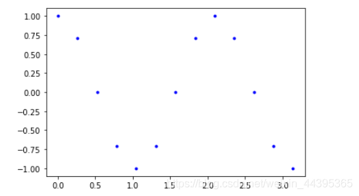
# 离散取值
a=np.arange(13)*pi/12
b=cos(3*a)
plot(a,b,'bo',markersize=3)
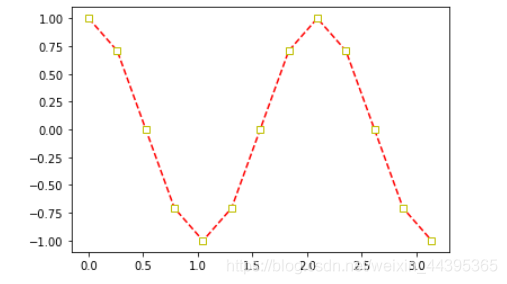
# 离散取值的属性及用虚线相连
a=np.arange(13)*pi/12
b=cos(3*a)
plot(a,b,'--rs',markeredgecolor='y',markerfacecolor='w')
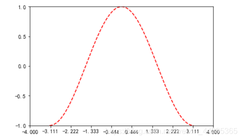
# 设置坐标轴的范围和记号
x=np.linspace(-pi,pi,256)
y,z=np.cos(x),np.sin(x)
xlim(-4,4)
xticks(np.linspace(-4,4,10))
ylim(-1.0,1.0)
yticks(np.linspace(-1.0,1.0,5))
plt.plot(x,y,'--r')
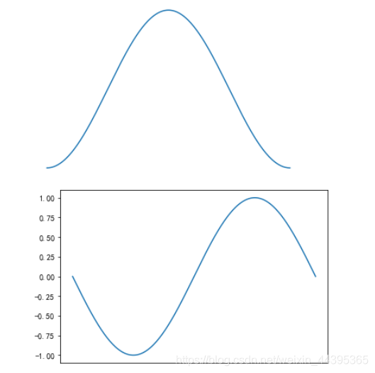
# 设置title与坐标轴的一些操作
# 设置中文
matplotlib.rcParams['axes.unicode_minus'] =False
plt.rcParams['font.sans-serif'] = ['SimHei']
x=np.linspace(-pi,pi,256)
y,z=np.cos(x),np.sin(x)
figure()
plt.plot(x,y)
axis('off')

figure()
plt.plot(x,z)
plt.xticks([])

plt.show()
# 设置title与坐标轴的一些操作
# 设置中文
matplotlib.rcParams['axes.unicode_minus'] =False
plt.rcParams['font.sans-serif'] = ['SimHei']
x=np.linspace(-pi,pi,256)
y,z=np.cos(x),np.sin(x)
figure()
plt.plot(x,y)
axis('off')

figure()
plt.plot(x,z)
plt.xticks([])

plt.show()
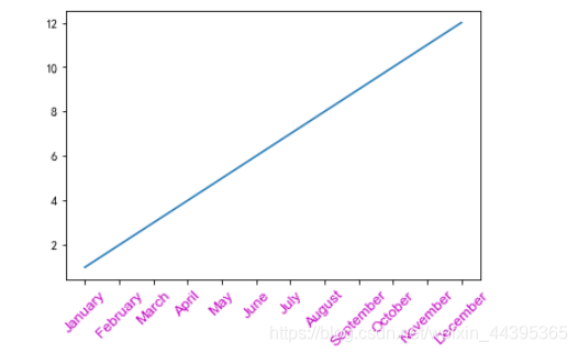
#设置坐标轴的标签(多样化)
# xticks(locs, [labels], **kwargs)  # Set locations and labels **kwargs是关键字参数
import calendar

x = range(1,13,1)
y = range(1,13,1)
plt.plot(x,y)
# 标签手动设置('','','',...)亦可
plt.xticks(x, calendar.month_name[1:13],color='m',rotation=45,fontsize=12,fontname='Arial')
plt.show()
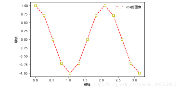
# 设置图例
matplotlib.rcParams['axes.unicode_minus'] =False

plt.rcParams['font.sans-serif'] = ['SimHei']
a=np.arange(13)*pi/12
b=cos(3*a)
plt.plot(a,b,'--rs',markeredgecolor='y',markerfacecolor='w',label='cos的图像')
xlabel('横轴')
ylabel('纵轴')
plt.legend(loc='upper right')
plt.show()
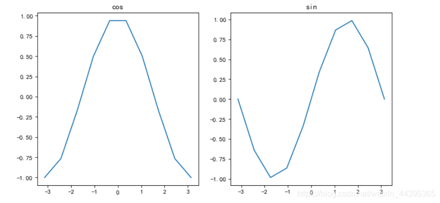
# 子图1
matplotlib.rcParams['axes.unicode_minus'] =False

x=np.linspace(-pi,pi,10)
y,z=np.cos(x),np.sin(x)
fig, (ax1 ,ax2) = plt.subplots(nrows=1, ncols=2, figsize=(8, 4))
ax1.plot(x,y),ax2.plot(x,z)
ax1.set_title('cos'),ax2.set_title('sin')
plt.show()
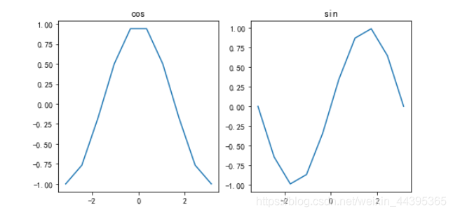
# 子图2
matplotlib.rcParams['axes.unicode_minus'] =False

x=np.linspace(-pi,pi,10)
y,z=np.cos(x),np.sin(x)
figure(figsize=(10,5),dpi=80)
subplot(121),plt.plot(x,y),plt.title('cos')
subplot(122),plt.plot(x,z),plt.title('sin')
plt.show()
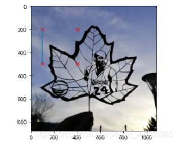
2.1 绘制实际图像中的点和线
# 使用matplotlib连线
from PIL import Image
from pylab import *

# 读取为列表,以便标记x、y的点?
im=array(Image.open('pic/kobe_mamba.jpg'))

imshow(im)

# 列表 包含四个点坐标
x=[100,100,400,400]
y=[200,500,200,500]

#红色叉型标出
plot(x,y,'rx')


# 连接坐标的前两个点的线 (100,200)与(100,500)
plot(x[:2],y[:2])

show()
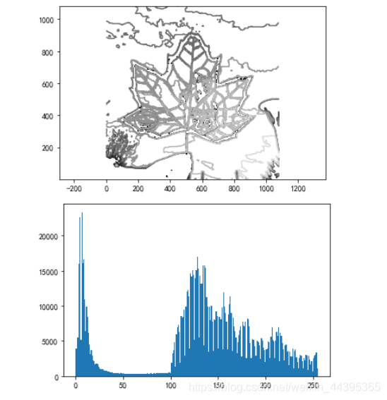
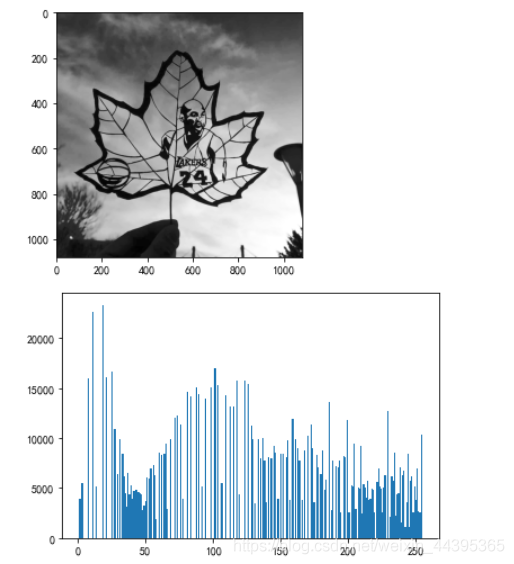
2.2 图像轮廓与直方图
# contour 与 hist
# 绘制轮廓要将图像先灰度化
from PIL import Image
from pylab import *

im=array(Image.open('pic/kobe_mamba.jpg').convert('L'))
figure()
#
gray()
# 绘制轮廓,且起始位置从左上角开始
contour(im,origin='image')

# 坐标轴均匀分布
axis('equal')

# 新图像
figure()
hist(im.ravel(),256)

# hist的第二个参数指定小区间的个数,128个,即每个小区间灰度值跨度为2
figure()
hist(im.flatten(),128)

show()
三、Numpy库基本学习
import numpy as np
import math
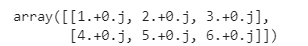
a=np.array(((1,2,3),(4,5,6)),dtype=float/complex)
a

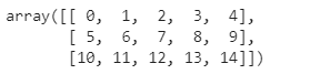
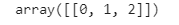
b=np.arange(15).reshape(3,5)
b
# 属性
b.shape
b.ndim
b.dtype
b.size
b.itemsize
from numpy import pi
np.linspace( 0, 2, 9 )                 # 9 numbers from 0 to 2
array([ 0.  ,  0.25,  0.5 ,  0.75,  1.  ,  1.25,  1.5 ,  1.75,  2.  ])
c=np.random.random((2,3))

c.max/min()
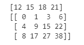
d=np.arange(12).reshape((3,4))
d.dtype.name
# 每个col的sum
print(d.sum(axis=0))
# 每行的累计和
print(d.cumsum(axis=1))
# 转变数组类型
a=np.array(((1,2,3),(4,5,6)),'float32')
a=a.astype('int16')
a

# 索引和切片
a = np.arange(10)**3 # 0~9的立方
a[2:5] #a[2-4]
# 令a[0,2,4]为-1000
a[:6:2] = -1000
# reverse
a[ : :-1]

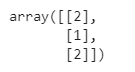
a = np.arange(12).reshape((3,4))
a[0:3,1]
# 第2列
# or
a[:,1]
a[0:1,0:3]
# 变换为1维数组
a = np.arange(12).reshape((3,4))
a.ravel()

# 变换形状
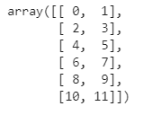
a = np.arange(12).reshape((3,4))
a.resize((6,2))
a
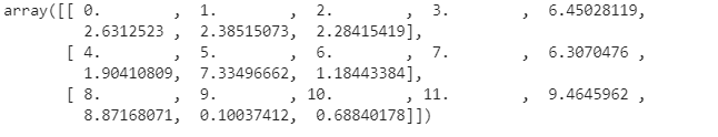
a = np.arange(12).reshape((3,4))
b=10*np.random.random((3,4))
# 竖着叠加
np.vstack((a,b))
# 横着叠加
np.hstack((a,b))
x, y = np.ogrid[:3, :4]
# 同样可以设置步长
x, y = np.ogrid[0:3:1, 0:5:2]

# 询问,x>0的部分不变,其余赋值为2
np.where(x>0,x,2)
3.1 直方图均衡化
# 解释累加函数
import numpy as np
a=[1,2,3,4,5,6,7]
cdf=np.cumsum(a)

cdf[-1]

cdf=7*cdf/cdf[-1]
cdf
28

# 直方图均衡化
# bins 小区间的个数
def histeq(im,bins=256):
    #返回两个参数
    imhist,bins=histogram(im.flatten(),bins)
    # 累计分布函数,相当于cdf是一个列表
    cdf=imhist.cumsum()
    # cdf[-1]是列表的最后一个值,(0,255)
    cdf=255*cdf/cdf[-1]
    # 新的线性插值
    im2=interp(im.flatten(),bins[:-1],cdf)
    # 返回im2图像大小与im相同
    return im2.reshape(im.shape),cdf
# 直方图先转为灰度图
im=array(Image.open('pic/kobe_mamba.jpg').convert('L'))
im2,cdf=histeq(im,256)

figure()
imshow(im2)
figure()
hist(im2.flatten(),256)
show()
3.2 图像缩放
#  转换为array
img = np.asarray(image)

# 转换为Image
Image.fromarray(np.uint8(img))

# 图像缩放函数

def imresize(im,sz):
    # 将数组转换为图像
    pil_im=Image.fromarray(np.uint8(im))
    # 图像转换为数组
    return np.array(pil_im.resize(sz))

imshow(imresize(Image.open('pic/kobe_mamba.jpg'),(128,128)))
3.3 图像的主成分分析(PCA)
PCA(Principal Component Analysis,主成分分析)是一个非常有用的降维技巧。它可以在使用尽可能少维数的前提下,尽量多地保持训练数据的信息,在此意义上是一个最佳技巧。即使是一幅 100×100 像素的小灰度图像,也有 10 000 维,可以看成 10 000 维空间中的一个点。一兆像素的图像具有百万维。由于图像具有很高的维数,在许多计算机视觉应用中,我们经常使用降维操作。PCA 产生的投影矩阵可以被视为将原始坐标变换到现有的坐标系,坐标系中的各个坐标按照重要性递减排列。
为了对图像数据进行 PCA 变换,图像需要转换成一维向量表示。我们可以使用 NumPy 类库中的flatten() 方法进行变换。
将变平的图像堆积起来,我们可以得到一个矩阵,矩阵的一行表示一幅图像。在计算主方向之前,所有的行图像按照平均图像进行了中心化。我们通常使用 SVD(Singular Value Decomposition,奇异值分解)方法来计算主成分;但当矩阵的维数很大时,SVD 的计算非常慢,所以此时通常不使用 SVD 分解。
from PIL import Image
from numpy import *

def pca(X):
  """ 主成分分析:
    输入:矩阵X ,其中该矩阵中存储训练数据,每一行为一条训练数据
    返回:投影矩阵(按照维度的重要性排序)、方差和均值"""

  # 获取维数
    num_data,dim = X.shape

  # 数据中心化
    mean_X = X.mean(axis=0)
    X = X - mean_X

if dim>num_data:
  # PCA- 使用紧致技巧
  M = dot(X,X.T) # 协方差矩阵
  e,EV = linalg.eigh(M) # 特征值和特征向量
  tmp = dot(X.T,EV).T # 这就是紧致技巧
  V = tmp[::-1] # 由于最后的特征向量是我们所需要的,所以需要将其逆转
  S = sqrt(e)[::-1] # 由于特征值是按照递增顺序排列的,所以需要将其逆转
  for i in range(V.shape[1]):
    V[:,i] /= S
else:
  # PCA- 使用SVD 方法
  U,S,V = linalg.svd(X)
  V = V[:num_data] # 仅仅返回前nun_data 维的数据才合理

# 返回投影矩阵、方差和均值
return V,S,mean_X
四、Scipy
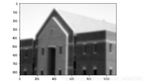
4.1 图像模糊
# 图像模糊
# Scipy 库
from PIL import Image
from numpy import *
from scipy.ndimage import filters

im=array(Image.open('pic/building.tif').convert('L'))
# filters.gaussian_filter第二个参数是标准差
im2=filters.gaussian_filter(im,9)
imshow(im2)
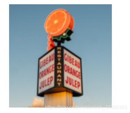
from PIL import Image
# 彩色通道,三通道分别进行高斯滤波
im=array(Image.open('pic/landmark500x500.jpg'))
im2=np.zeros((im.shape))
for i in arange(3):
    im2[:,:,i]=filters.gaussian_filter(im[:,:,i],2)

# 转换为(0,255),否则imshow显示不出来
im2=uint8(im2)
figure(figsize=(5,5),dpi=80)
imshow(im2)
axis('off')
4.2 图像导数
from PIL import Image
from numpy import *
from scipy.ndimage import filters

# filters.sobel(src,0/1,dst),0表示y方向的方向导数,1表示x方向的方向导数

figure()
im=array(Image.open('pic/building.tif'))
imshow(im)


imx=np.zeros(im.shape)

imy=np.zeros(im.shape)
filters.sobel(im,0,imy)
figure()
imx=uint8(imy)
imshow(imy)

figure()
filters.sobel(im,1,imx)
imy=uint8(imx)
imshow(imx)

figure()
mag=sqrt(imx**2+imy**2)
mag=uint8(mag)
imshow(mag)

show()
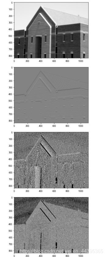
第二/三张图是sobel算子在x/y方向的导数,第四张图是两个导数叠加成梯度。
4.3 形态学计数
# 形态学 对象计数
from scipy.ndimage import measurements,morphology

im=array(Image.open('pic/zhiwen.tif').convert('L'))
im2=np.zeros(im.shape)
im2=1*(im128)

labels,nbr_objects=measurements.label(im2)

print(f"Number of objects is {nbr_objects}.")

labels=np.uint8(labels)
imshow(labels)

im_open=morphology.binary_opening(im2,ones((3,3)),1)
labels_open,nbr_objects_open=measurements.label(im_open)
print(f"Number of objects is {nbr_objects_open}.")

imshow(labels_open)
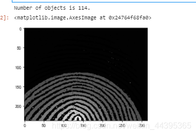
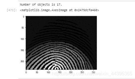
形态学计数使用label()函数,令图像的灰度值为标签,图一找到了114个物体,图二经过开操作,找到了17个物体。
到此这篇关于Python一些基本的图像操作和处理总结的文章就介绍到这了,更多相关Python图像操作和处理内容请搜索脚本之家以前的文章或继续浏览下面的相关文章希望大家以后多多支持脚本之家!
您可能感兴趣的文章:- 使用Python给头像戴上圣诞帽的图像操作过程解析
- Python用Pillow(PIL)进行简单的图像操作方法
- 2021年最新用于图像处理的Python库总结
- python图像处理基本操作总结(PIL库、Matplotlib及Numpy)
- Python图像处理之膨胀与腐蚀的操作
- python opencv图像处理(素描、怀旧、光照、流年、滤镜 原理及实现)


 咨 询 客 服